Direct Image® Operational Tips Email

In this issue we are highlighting:

• Direct Image® Software Release V3.3
• HPT Controller Upgrade
• Locating DNAPL with MIP
• Come and visit us at the Battelle Symposium

DI Viewer and Acquisition V3.3 Release:

Geoprobe® Direct Image® has released the latest update on DI Software. The latest version of software can be downloaded from: https://geoprobe.com/direct-image-software-downloads

DI Acquisition V3.3 Improvements:

• Improved installation which includes: Added a code signing certificate within the installer security window. This shows the installer (Viewer and Acquisition) is from Geoprobe® – a trusted software source.
• The installer checks your system for the necessary .NET framework 4.6.1 required for proper operation.
• Addition of MIHPT-CPT, OIHPT-CPT and OIHPT-G in the probe selection option menu depending upon the mode of operation.
• Addition of a probe serial number text box on the probe selection screen. This will allow for better tracking of probe footage.
• Updated drivers for OIP logging.
• Improved OIP alarms
• Added a COM port debugging tool for troubleshooting communication issues. Accessed under Tools function tab.

Figure 1: OIP Log showing display of images from multiple log depths.

DI Viewer V3.3 Improvements:

• Multiple image display in OIP modes (Figure 1, above)
• Modification of the observed fluorescence graph label on OIP logs to identify the image filter being used.

geoprobe.com/direct-image-software-downloads

HPT Controller Upgrade:

In early 2017, we changed some of the components in the HPT Pump and controller. These changes provide better pump performance, longer pump life, and easier maintenance. These changes include:  

• Replacing the aluminum block manifold to a high-pressure plastic manifold (1) reducing corrosion and reaction with the water injected.
• Moving the in-line water filter from inside the box to being accessible from the back panel (2).
• Changing the bypass valve seats from brass to stainless steel (3). This reduces corrosion and leakage.

These improvements will reduce the amount of internal corrosion, pitting and generation of flocculants from reaction with water remaining in the HPT manifold. It also makes cleaning the filter far easier since it can be easily accessed from the back panel. These improvements may help the upcoming HPT field season go smoother and prevent undesirable and costly downtime.

Contact Geoprobe® Direct Image® for a cost estimate to upgrade your HPT pump with these improved features.

Identifying DNAPL using MIP:

A significant amount of MIP work is performed to delineate chlorinated solvent plumes and determine their sources. This may include encountering a DNAPL source whether it is expected or not. Here are the indicators within the MIP graphs that can lead us to the most likely locations on a site where DNAPL may be found.

MIP Log DNAPL Identifiers and Operational tips:

1. High MIP detector signal levels can indicate the presence of NAPL. Here are some example values for TCE:

2. These are example MIP detector responses for TCE run on a MIP detector system at Geoprobe®.
3. Look for low spots in basal silt and clay formations in the EC-HPT data where DNAPL may collect.
4. Compare cross sectional responses of all detector data and make sure you observe the FID response which will show the greatest contrast between DNAPL and high dissolved phase responses. The FID can highlight the area where DNAPL is located.
5. MIP pressure may show a very slight increase in pressure after DNAPL has diffused through the membrane and is on its way to the detectors.
6. Ensure that you are operating your detector in medium or preferably low gain setting with appropriate attenuation factors in the software prior to advancing the MIP tools into areas of likely DNAPL.
7. Do not use ECD data for high concentration CVOCs

Below we will explain these points further:

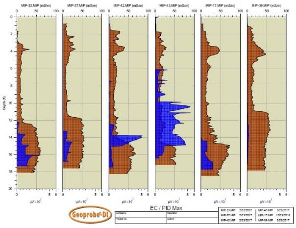
(1) Based upon the data we have seen and collected, when your detector (PID, XSD and FID) responses are reaching into the 107 μV levels there is a good probability DNAPL will be present.

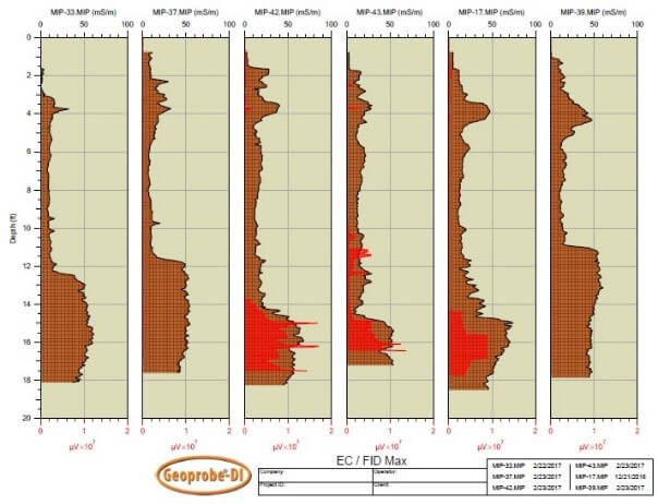
(2) Here are cross sectional displays of a series of logs (EC and MIP detector graphs). Notice the sand-till contact is deeper on the EC graph (brown fill) in the 3rd to 5th logs from the left. This will act as a DNAPL point of collection. The XSD (green fill) and PID (blue fill) both show higher responses in the 3rd to 5th logs but also have visible signal in adjacent logs at these scales.

(3) The FID (red) displays a much higher signal in the TCE DNAPL compared to the dissolved phase adjacent to it. This higher FID signal helps to pinpoint the location of DNAPL in the cross section.

(4) During this study, we observed the MIP pressure graph may show a slight rise in pressure during this study that when the membrane is exposed to DNAPL. This is a result of NAPL increasing the vapor density of carrier gas stream as it moves through the trunkline to the detectors. This observation requires a very stable MIP pressure prior to encountering the DNAPL zone. This can be seen in the graphs below:

Slight increase in MIP pressure when NAPL is encountered.

(5) Expecting DNAPL? Adjust your detector gain settings to low (SRI -PID, FID and OI XSD with appropriate attenuation setting) prior to beginning the log. At these levels you would not need to change them in the ground. You might start out with a bit more detector signal noise, but this will not matter once you reach high dissolved phase concentrations and beyond.

Gain/Attenuation Settings on the GC detectors and the DI Acquisition software
 

GC Gain/Range settings and associated software multipliers. 

The detectors controlled by HP GC have been observed to require using a detector range of 7 and attenuation factor of 128 in LNAPL plumes. For chlorinated DNAPL, it would be recommended to start the log using a range of 5 or 6 and 32 or 64 on the attenuation to reduce likelihood of an in-ground change. These steps do not need to be done incrementally. More information on using MIP to identify DNAPL can be found here.

Battelle Symposium:

Come visit us at the Battelle Symposium in Baltimore, MD April 15th-18th
Geoprobe® Direct Image® at Booth 514
Wes McCall, Adam McMath, and Dan Pipp

https://geoprobe.com/geoprobe-direct-image