Lower your MIP detection limits and increase your system usage with the LL MIP Pulse Flow controller
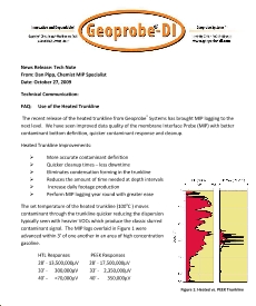
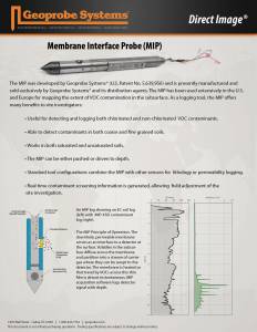
LL MIP was developed as a way to reduce MIP VOCS detection limits and offers the capability of reaching well below 100ppb total VOCS. These lowered VOCS detection limits means operators equipment sees more days in the field as plume investigations go to further extents and sites that MIP equipment would previously not have been used on are being investigated.
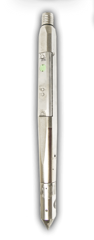
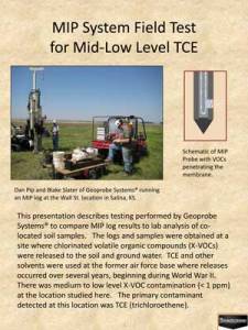
= Tool String Diagram (TSD)
System Overview
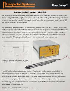
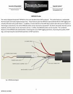
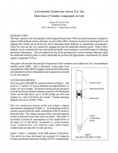
Low Level MIP (LL MIP) is a technology developed by Geoprobe Systems® that greatly increases the sensitivity (and therefore utility) of the MIP logging tool. The primary feature of LL MIP technology is that the carrier gas stream that sweeps the internal surface of the MIP membrane is pulsed. This results in an increase in the concentration of VOC contaminant delivered to the MIP detectors.
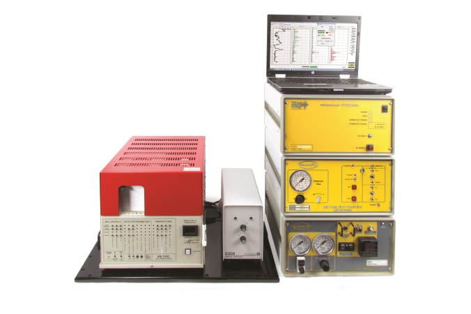
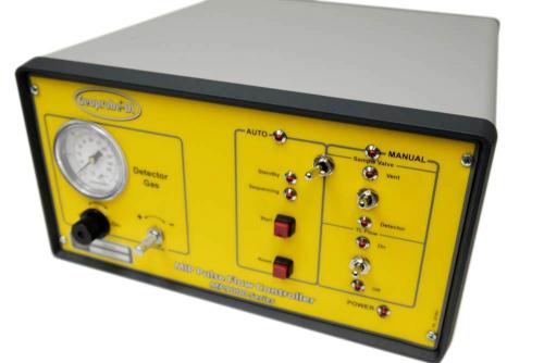
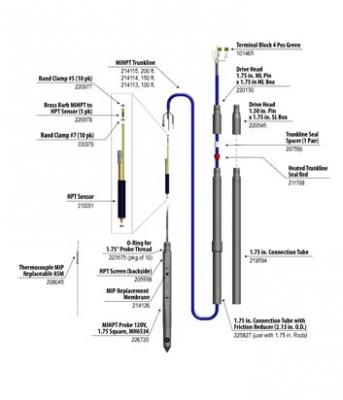
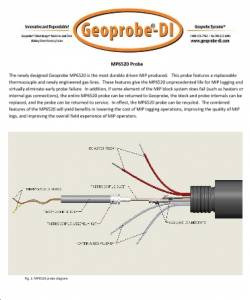
Low Level MIP can be performed with any style of MIP probes or trunkline. To perform this method an operator will need to add the MP9000 Pulse Flow Controller (Figure 1) to their current MIP system and be using a current version of DI Acquisition software. The addition of the MP9000 to the system is simple and requires only the rearrangement of gas line connections. This controller can then be easily removed from the system to return to standard MIP logging. Switching between methods requires only a few minutes of time.
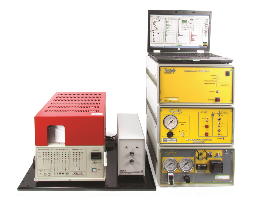
Figure 1:
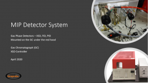
LL MIP Equipment: GC and detectors, FI6000, MP9000, MP6505
General Operation:
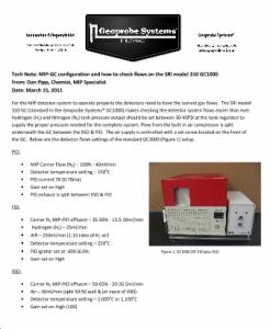
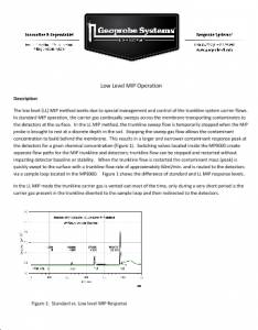
In standard MIP operation, the carrier gas continually sweeps across the membrane transporting contaminates to the detectors at the surface. In the LL MIP method, the trunkline sweep flow is temporarily stopped when the MIP probe is brought to rest at a discrete depth in the soil. Stopping the sweep gas flow allows the contaminant concentration to build behind the membrane. This results in a larger and narrower contaminant response peak at the detectors (Fig. 2 and 3) for a given chemical concentration. Switching valves located inside the MP9000 create separate flow paths for the MIP trunkline and detectors; trunkline flow can be stopped and restarted without impacting detector baseline or stability. When the trunkline flow is restarted the contaminant mass (peak) is quickly swept to the surface with a trunkline flow rate of approximately 60ml/min. and is routed to the detectors via the MP9000.
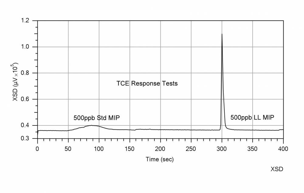
Figure 2:
Comparison of 0.5ppm Trichloroethylene response between standard MIP (50s-100s) and Low Level MIP (300s) methods
The Low Level MIP operation is automated in DI Acquisition software version 3.0 or newer which controls the timed cycling of the MP9000 controller. This software includes a subroutine for automatic triggering of LL MIP cycling at preset depth intervals during the MIP logging process.
The LL MIP method will greatly increase the sensitivity of a MIP system but the resulting detection limits are dependent on the sensitivity of the standard MIP system. To achieve the lowest possible detection limits the probe and trunkline need to be new or verified clean with system blanks. The detectors also need to be fully current within their maintenance program and sensitivity should be tested prior to mobilization. Equipment that has been used to map high level contaminants will result in false positive results due to contaminant desorption from the membrane and return carrier gas line.
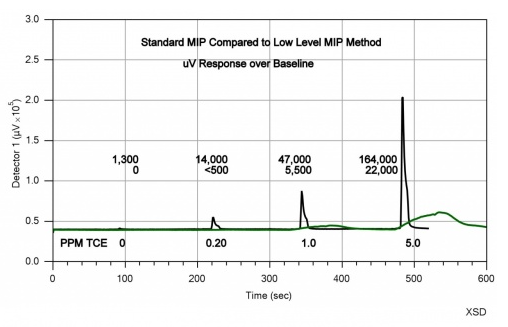
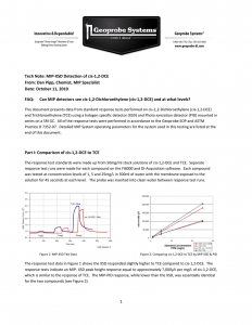
Figure 3:
Comparison of 0.2, 1.0, and 5.0ppm Trichloroethylene in standard and LL MIP methods
Example Logs
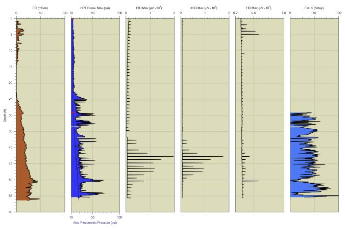
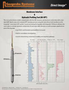
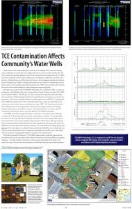
The LL MIHPT Log in Figure 4 shows a highly permeable likely sandy formation in the top 22ft as indicated by the low EC and HPT pressure values. Permeability stays fairly low throughout the log with occasional layers of lower permeability. The predominant contaminant is seen from approximately 37ft to 51ft and is detected primarily on the PID and XSD. Since the compounds respond on the XSD we know them to contain halogenated probably double bonded halogenated due to the PID confirmation, which to respond on the PID requires an ionization potential below the lamps 10.6eV. The halogenated compounds that have lower ionization potential are typically double bonded chemicals. The FID shows some responses within the first 5ft of the log which the other detectors do not confirm. This is a common trait of natural gas or methane deposits which is non-halogenated and has a higher ionization potential than the lamp. In the lower contaminant zone there is a confirmed response on the FID although lower in magnitude than the PID and XSD due to the lower sensitivity of the FID for these compounds. Another item to note is that the PID displays consistent responses throughout the log, if it quite common for the PID to provide a background level response in LL MIP mode and the lower responses must be disregarded.
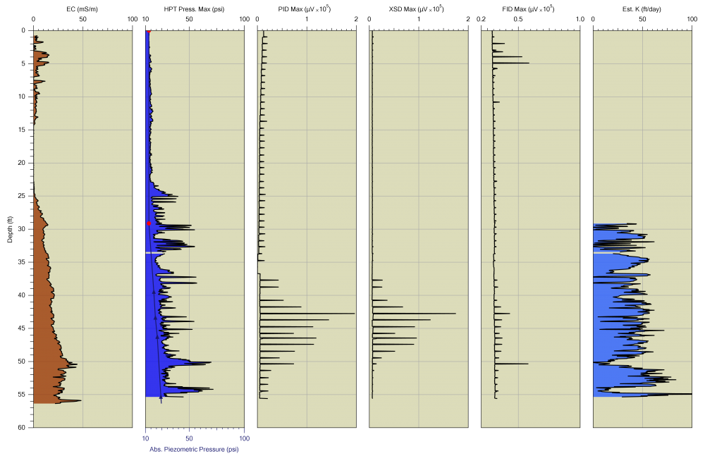
Figure 4:
LL MIHPT Log displaying graphs (left to right) EC, HPT Pressure (primary axis), Piezeometric profile (secondary axis), MIP-PID, XSD, FID, and Est. K.
The LL MIHPT Log in Figure 5 shows a lowery permeability soils such as silts and clays in the top 45ft as indicated by the higher EC and HPT pressure values. This site breaks into a sandy formation below 45ft indicated by the lower EC and HPT pressure below this point. The predominant contaminant is seen from approximately 15ft to 33ft and is detected primarily on the PID and FID with no XSD response. Since there is no response on the XSD we know it is a non-halogenated compound. This log came from a former fuel service station so the PID and FID response likely is aromatic and nonaromatic fuel hydrocarbons.
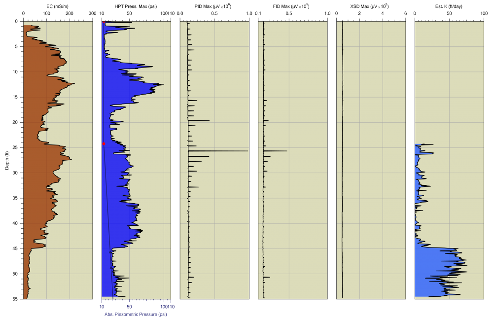
Figure 5:
LL MIHPT Log displaying graphs (left to right) EC, HPT Pressure (primary axis), Piezeometric profile (secondary axis), MIP-PID, FID, XSD, and Est. K.
The LL MIHPT Log in Figure 6 shows a lower permeable clay at the top 5ft transitioning into likely a sandy silt formation down to 30ft as indicated by the low EC and HPT pressure values. Below 30ft the formation is a fairly clean sand with low EC and HPT values. Permeability stays low throughout the log with occasional layers of lower permeability below 50ft. There are different contaminants in this log with likely petroleum hydrocarbons in the top 30ft responding on the PID and FID only but then the XSD shows halogenated compounds 35ft-42ft and again from 52ft to the end of the boring. These XSD responses are not confirmed on the PID which indicates that the ionization potential is likely too high for the PID to detect. This typically occurs with single bonded halogenated compounds. Confirmation groundwater samples were taken from these locations and 1,2-Dichloroethane was the predominant contaminant in the zone from 35ft to 42ft, in the lower section it was mostly Chloroform and Carbon Tetrachloride. All of these compounds have ionization potentials over 11eV, so they would not be detected by the PID.
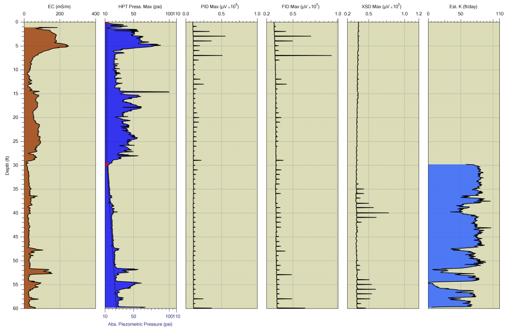
Figure 6:
LL MIHPT Log displaying graphs (left to right) EC, HPT Pressure (primary axis), Piezeometric profile (secondary axis), MIP-PID, FID, XSD, and Est. K.
MIP Method Comparison
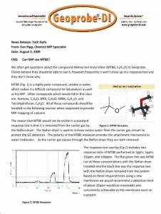
Low level MIP will not replace standard MIP logging, but will expand MIP capabilities. LL MIP is most useful when low contaminant concentrations are present. Figure 7 displays an overlay of closely spaced standard MIP and LL MIP logs at locations of lower concentration petroleum and chlorinated VOC’s. The LL MIP log exhibits robust signal to noise and the presence and location of contamination is easily defined. The standard MIP log you might be able to discern there is a contaminant if you zoom in on the baseline but at times you can wonder if the basleine movement is due to contaminant or is detector baseline drift. This log displays petroleum hydrocarbon presence in the top half of the log with PID-FID responses and no XSD response and in the lower half of the log there are chlorinated contamoinants present as displayed by the PID-XSD responses. Projects with contaminant concentrations too low to proceed with traditional MIP methods may be good candidates for investigation using the LL MIP method. This technology will provide operators with the ability to track and map contaminant plumes down to concentrations at or below the 100ppb range for some contaminants.
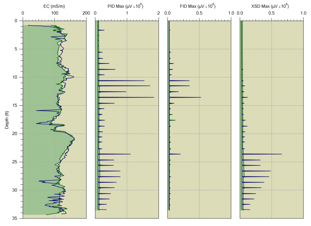
Figure 7:
Collocated standard (shaded green) and LL MIP Logs overlaid displaying (left to right) EC, MIP-PID, FID, and XSD
The MIP logs compared in Figure 8 display closely spaced standard and LL MIP logs at locations of lower concentration chlorinated VOC’s. While it is difficult or even impossible to discern the presence of VOC contamination based on the standard MIP log at this location, the LL MIP log exhibits robust signal to noise and the presence and location of contamination is easily defined.
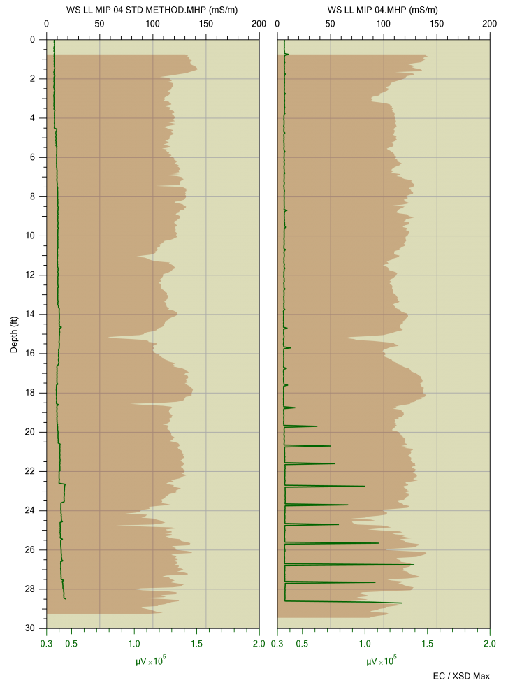
Figure 8:
Collocated standard and LL MIP Logs displaying EC (shaded brown) and XSD (green)
The MIP logs compared in Figure 9 again display closely spaced standard and LL MIP logs at locations of lower concentration chlorinated VOC’s. The standard MIP log at this location is a bit easier to discern that contaminantes are likely present in this log however the LL MIP log displays strong signal to noise and the presence and location of contamination is easily defined.
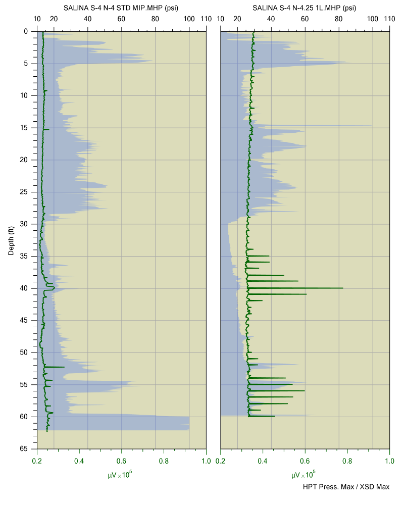
Figure 9:
Collocated standard and LL MIP Logs displaying HPT Pressure (shaded blue) and XSD (green)
Features & Options
LL MIP Pulse Flow Controller
Low Level MIP (LL MIP) is a technology developed by Geoprobe Systems® that greatly increases the sensitivity (and therefore utility) of the MIP logging tool. The primary feature of LL MIP technology is that the carrier gas stream that sweeps the internal surface of the MIP membrane is pulsed. This results in an increase in the concentration of VOC contaminant delivered to the MIP detectors.
Low Level MIP can be performed with any style of MIP probes or trunkline. To perform this method an operator will need to add the MP9000 Pulse Flow Controller (Figure 1) to their current MIP system and be using a current version of DI Acquisition software. The addition of the MP9000 to the system is simple and requires only the rearrangement of gas line connections. This controller can then be easily removed from the system to return to standard MIP logging. Switching between methods requires only a few minutes of time.
Figure 1:
LL MIP Equipment: GC and detectors, FI6000, MP9000, MP6505
General Operation:
In standard MIP operation, the carrier gas continually sweeps across the membrane transporting contaminates to the detectors at the surface. In the LL MIP method, the trunkline sweep flow is temporarily stopped when the MIP probe is brought to rest at a discrete depth in the soil. Stopping the sweep gas flow allows the contaminant concentration to build behind the membrane. This results in a larger and narrower contaminant response peak at the detectors (Fig. 2 and 3) for a given chemical concentration. Switching valves located inside the MP9000 create separate flow paths for the MIP trunkline and detectors; trunkline flow can be stopped and restarted without impacting detector baseline or stability. When the trunkline flow is restarted the contaminant mass (peak) is quickly swept to the surface with a trunkline flow rate of approximately 60ml/min. and is routed to the detectors via the MP9000.
Figure 2:
Comparison of 0.5ppm Trichloroethylene response between standard MIP (50s-100s) and Low Level MIP (300s) methods
The Low Level MIP operation is automated in DI Acquisition software version 3.0 or newer which controls the timed cycling of the MP9000 controller. This software includes a subroutine for automatic triggering of LL MIP cycling at preset depth intervals during the MIP logging process.
The LL MIP method will greatly increase the sensitivity of a MIP system but the resulting detection limits are dependent on the sensitivity of the standard MIP system. To achieve the lowest possible detection limits the probe and trunkline need to be new or verified clean with system blanks. The detectors also need to be fully current within their maintenance program and sensitivity should be tested prior to mobilization. Equipment that has been used to map high level contaminants will result in false positive results due to contaminant desorption from the membrane and return carrier gas line.
Figure 3:
Comparison of 0.2, 1.0, and 5.0ppm Trichloroethylene in standard and LL MIP methods
The LL MIHPT Log in Figure 4 shows a highly permeable likely sandy formation in the top 22ft as indicated by the low EC and HPT pressure values. Permeability stays fairly low throughout the log with occasional layers of lower permeability. The predominant contaminant is seen from approximately 37ft to 51ft and is detected primarily on the PID and XSD. Since the compounds respond on the XSD we know them to contain halogenated probably double bonded halogenated due to the PID confirmation, which to respond on the PID requires an ionization potential below the lamps 10.6eV. The halogenated compounds that have lower ionization potential are typically double bonded chemicals. The FID shows some responses within the first 5ft of the log which the other detectors do not confirm. This is a common trait of natural gas or methane deposits which is non-halogenated and has a higher ionization potential than the lamp. In the lower contaminant zone there is a confirmed response on the FID although lower in magnitude than the PID and XSD due to the lower sensitivity of the FID for these compounds. Another item to note is that the PID displays consistent responses throughout the log, if it quite common for the PID to provide a background level response in LL MIP mode and the lower responses must be disregarded.
Figure 4:
LL MIHPT Log displaying graphs (left to right) EC, HPT Pressure (primary axis), Piezeometric profile (secondary axis), MIP-PID, XSD, FID, and Est. K.
The LL MIHPT Log in Figure 5 shows a lowery permeability soils such as silts and clays in the top 45ft as indicated by the higher EC and HPT pressure values. This site breaks into a sandy formation below 45ft indicated by the lower EC and HPT pressure below this point. The predominant contaminant is seen from approximately 15ft to 33ft and is detected primarily on the PID and FID with no XSD response. Since there is no response on the XSD we know it is a non-halogenated compound. This log came from a former fuel service station so the PID and FID response likely is aromatic and nonaromatic fuel hydrocarbons.
Figure 5:
LL MIHPT Log displaying graphs (left to right) EC, HPT Pressure (primary axis), Piezeometric profile (secondary axis), MIP-PID, FID, XSD, and Est. K.
The LL MIHPT Log in Figure 6 shows a lower permeable clay at the top 5ft transitioning into likely a sandy silt formation down to 30ft as indicated by the low EC and HPT pressure values. Below 30ft the formation is a fairly clean sand with low EC and HPT values. Permeability stays low throughout the log with occasional layers of lower permeability below 50ft. There are different contaminants in this log with likely petroleum hydrocarbons in the top 30ft responding on the PID and FID only but then the XSD shows halogenated compounds 35ft-42ft and again from 52ft to the end of the boring. These XSD responses are not confirmed on the PID which indicates that the ionization potential is likely too high for the PID to detect. This typically occurs with single bonded halogenated compounds. Confirmation groundwater samples were taken from these locations and 1,2-Dichloroethane was the predominant contaminant in the zone from 35ft to 42ft, in the lower section it was mostly Chloroform and Carbon Tetrachloride. All of these compounds have ionization potentials over 11eV, so they would not be detected by the PID.
Figure 6:
LL MIHPT Log displaying graphs (left to right) EC, HPT Pressure (primary axis), Piezeometric profile (secondary axis), MIP-PID, FID, XSD, and Est. K.
Low level MIP will not replace standard MIP logging, but will expand MIP capabilities. LL MIP is most useful when low contaminant concentrations are present. Figure 7 displays an overlay of closely spaced standard MIP and LL MIP logs at locations of lower concentration petroleum and chlorinated VOC’s. The LL MIP log exhibits robust signal to noise and the presence and location of contamination is easily defined. The standard MIP log you might be able to discern there is a contaminant if you zoom in on the baseline but at times you can wonder if the basleine movement is due to contaminant or is detector baseline drift. This log displays petroleum hydrocarbon presence in the top half of the log with PID-FID responses and no XSD response and in the lower half of the log there are chlorinated contamoinants present as displayed by the PID-XSD responses. Projects with contaminant concentrations too low to proceed with traditional MIP methods may be good candidates for investigation using the LL MIP method. This technology will provide operators with the ability to track and map contaminant plumes down to concentrations at or below the 100ppb range for some contaminants.
Figure 7:
Collocated standard (shaded green) and LL MIP Logs overlaid displaying (left to right) EC, MIP-PID, FID, and XSD
The MIP logs compared in Figure 8 display closely spaced standard and LL MIP logs at locations of lower concentration chlorinated VOC’s. While it is difficult or even impossible to discern the presence of VOC contamination based on the standard MIP log at this location, the LL MIP log exhibits robust signal to noise and the presence and location of contamination is easily defined.
Figure 8:
Collocated standard and LL MIP Logs displaying EC (shaded brown) and XSD (green)
The MIP logs compared in Figure 9 again display closely spaced standard and LL MIP logs at locations of lower concentration chlorinated VOC’s. The standard MIP log at this location is a bit easier to discern that contaminantes are likely present in this log however the LL MIP log displays strong signal to noise and the presence and location of contamination is easily defined.
Figure 9:
Collocated standard and LL MIP Logs displaying HPT Pressure (shaded blue) and XSD (green)
The data generated from the LL MIHPT survey provided much more certainty on the permeable reactive barrier (PRB) needed to address the plume of contaminated groundwater migrating onto the client's property. Had the original design been followed, money would have been wasted in extending the PRB to areas of the site where it wasn't needed, and the deeper VOCS plume would have been completely missed. The refined PRB design resulted in a savings to the client of about 2.5 times the cost of the LL MIPHT survey, while at the same time avoiding failure by ensuring that the entire VOCS contaminant plume was captured by the PRB.
- Patrick O'Neill, Project Manager, Vertex Environmental Inc, Ontario, Canada
Videos
Resources
Click on a section below to view information.


Depend on Team Geoprobe®
Since 1987, Geoprobe® has manufactured innovative drilling rigs and tooling - engineered for efficiency and safety - simplifying drillers’ jobs and empowering their companies to succeed as productive and profitable leaders in the industry. When you partner with Geoprobe® you receive:
Customer-inspired Innovation
Engineering and building industry-leading drilling rigs, tooling, and techniques for the technical driller based on your needs to work safer and more efficiently.
Exceptional Value
Ensuring drilling rigs and tooling are created in conjunction – with consistent quality – to collect the highest-quality information with the most accurate result to get you to, into, and through the job efficiently.
Superior Service
Equipping you to do your best job and keeping you in the field via one-on-one expert sales and service technicians manning live support phone lines, shipping necessary parts same-day.
Low Level MIP (LL MIP) is a technology developed by Geoprobe Systems® that greatly increases the sensitivity (and therefore utility) of the MIP logging tool. The primary feature of LL MIP technology is that the carrier gas stream that sweeps the internal surface of the MIP membrane is pulsed. This results in an increase in the concentration of VOC contaminant delivered to the MIP detectors.
Low Level MIP can be performed with any style of MIP probes or trunkline. To perform this method an operator will need to add the MP9000 Pulse Flow Controller (Figure 1) to their current MIP system and be using a current version of DI Acquisition software. The addition of the MP9000 to the system is simple and requires only the rearrangement of gas line connections. This controller can then be easily removed from the system to return to standard MIP logging. Switching between methods requires only a few minutes of time.
Figure 1: LL MIP Equipment: GC and detectors, FI6000, MP9000, MP6505
General Operation:
In standard MIP operation, the carrier gas continually sweeps across the membrane transporting contaminates to the detectors at the surface. In the LL MIP method, the trunkline sweep flow is temporarily stopped when the MIP probe is brought to rest at a discrete depth in the soil. Stopping the sweep gas flow allows the contaminant concentration to build behind the membrane. This results in a larger and narrower contaminant response peak at the detectors (Fig. 2 and 3) for a given chemical concentration. Switching valves located inside the MP9000 create separate flow paths for the MIP trunkline and detectors; trunkline flow can be stopped and restarted without impacting detector baseline or stability. When the trunkline flow is restarted the contaminant mass (peak) is quickly swept to the surface with a trunkline flow rate of approximately 60ml/min. and is routed to the detectors via the MP9000.
Figure 2: Comparison of 0.5ppm Trichloroethylene response between standard MIP (50s-100s) and Low Level MIP (300s) methods
The Low Level MIP operation is automated in DI Acquisition software version 3.0 or newer which controls the timed cycling of the MP9000 controller. This software includes a subroutine for automatic triggering of LL MIP cycling at preset depth intervals during the MIP logging process.
The LL MIP method will greatly increase the sensitivity of a MIP system but the resulting detection limits are dependent on the sensitivity of the standard MIP system. To achieve the lowest possible detection limits the probe and trunkline need to be new or verified clean with system blanks. The detectors also need to be fully current within their maintenance program and sensitivity should be tested prior to mobilization. Equipment that has been used to map high level contaminants will result in false positive results due to contaminant desorption from the membrane and return carrier gas line.
Figure 3: Comparison of 0.2, 1.0, and 5.0ppm Trichloroethylene in standard and LL MIP methods
:
The LL MIHPT Log in Figure 4 shows a highly permeable likely sandy formation in the top 22ft as indicated by the low EC and HPT pressure values. Permeability stays fairly low throughout the log with occasional layers of lower permeability. The predominant contaminant is seen from approximately 37ft to 51ft and is detected primarily on the PID and XSD. Since the compounds respond on the XSD we know them to contain halogenated probably double bonded halogenated due to the PID confirmation, which to respond on the PID requires an ionization potential below the lamps 10.6eV. The halogenated compounds that have lower ionization potential are typically double bonded chemicals. The FID shows some responses within the first 5ft of the log which the other detectors do not confirm. This is a common trait of natural gas or methane deposits which is non-halogenated and has a higher ionization potential than the lamp. In the lower contaminant zone there is a confirmed response on the FID although lower in magnitude than the PID and XSD due to the lower sensitivity of the FID for these compounds. Another item to note is that the PID displays consistent responses throughout the log, if it quite common for the PID to provide a background level response in LL MIP mode and the lower responses must be disregarded.
Figure 4: LL MIHPT Log displaying graphs (left to right) EC, HPT Pressure (primary axis), Piezeometric profile (secondary axis), MIP-PID, XSD, FID, and Est. K.
The LL MIHPT Log in Figure 5 shows a lowery permeability soils such as silts and clays in the top 45ft as indicated by the higher EC and HPT pressure values. This site breaks into a sandy formation below 45ft indicated by the lower EC and HPT pressure below this point. The predominant contaminant is seen from approximately 15ft to 33ft and is detected primarily on the PID and FID with no XSD response. Since there is no response on the XSD we know it is a non-halogenated compound. This log came from a former fuel service station so the PID and FID response likely is aromatic and nonaromatic fuel hydrocarbons.
Figure 5: LL MIHPT Log displaying graphs (left to right) EC, HPT Pressure (primary axis), Piezeometric profile (secondary axis), MIP-PID, FID, XSD, and Est. K.
The LL MIHPT Log in Figure 6 shows a lower permeable clay at the top 5ft transitioning into likely a sandy silt formation down to 30ft as indicated by the low EC and HPT pressure values. Below 30ft the formation is a fairly clean sand with low EC and HPT values. Permeability stays low throughout the log with occasional layers of lower permeability below 50ft. There are different contaminants in this log with likely petroleum hydrocarbons in the top 30ft responding on the PID and FID only but then the XSD shows halogenated compounds 35ft-42ft and again from 52ft to the end of the boring. These XSD responses are not confirmed on the PID which indicates that the ionization potential is likely too high for the PID to detect. This typically occurs with single bonded halogenated compounds. Confirmation groundwater samples were taken from these locations and 1,2-Dichloroethane was the predominant contaminant in the zone from 35ft to 42ft, in the lower section it was mostly Chloroform and Carbon Tetrachloride. All of these compounds have ionization potentials over 11eV, so they would not be detected by the PID.
Figure 6: LL MIHPT Log displaying graphs (left to right) EC, HPT Pressure (primary axis), Piezeometric profile (secondary axis), MIP-PID, FID, XSD, and Est. K.
:
Low level MIP will not replace standard MIP logging, but will expand MIP capabilities. LL MIP is most useful when low contaminant concentrations are present. Figure 7 displays an overlay of closely spaced standard MIP and LL MIP logs at locations of lower concentration petroleum and chlorinated VOC’s. The LL MIP log exhibits robust signal to noise and the presence and location of contamination is easily defined. The standard MIP log you might be able to discern there is a contaminant if you zoom in on the baseline but at times you can wonder if the basleine movement is due to contaminant or is detector baseline drift. This log displays petroleum hydrocarbon presence in the top half of the log with PID-FID responses and no XSD response and in the lower half of the log there are chlorinated contamoinants present as displayed by the PID-XSD responses. Projects with contaminant concentrations too low to proceed with traditional MIP methods may be good candidates for investigation using the LL MIP method. This technology will provide operators with the ability to track and map contaminant plumes down to concentrations at or below the 100ppb range for some contaminants.
Figure 7: Collocated standard (shaded green) and LL MIP Logs overlaid displaying (left to right) EC, MIP-PID, FID, and XSD
The MIP logs compared in Figure 8 display closely spaced standard and LL MIP logs at locations of lower concentration chlorinated VOC’s. While it is difficult or even impossible to discern the presence of VOC contamination based on the standard MIP log at this location, the LL MIP log exhibits robust signal to noise and the presence and location of contamination is easily defined.
Figure 8: Collocated standard and LL MIP Logs displaying EC (shaded brown) and XSD (green)
The MIP logs compared in Figure 9 again display closely spaced standard and LL MIP logs at locations of lower concentration chlorinated VOC’s. The standard MIP log at this location is a bit easier to discern that contaminantes are likely present in this log however the LL MIP log displays strong signal to noise and the presence and location of contamination is easily defined.
Figure 9: Collocated standard and LL MIP Logs displaying HPT Pressure (shaded blue) and XSD (green)
: